github/digital_video_introduction

Fork 0

mirror of https://github.com/leandromoreira/digital_video_introduction.git synced 2026-01-08 22:18:10 -05:00

Files

Emil Santurio 7f1020a734 First part of "Removing redundancies"

2023-09-01 19:25:46 -03:00

67 KiB

Raw Blame History

🇺🇸 🇨🇳 🇯🇵 🇮🇹 🇰🇷 🇷🇺 🇧🇷 🇪🇸

Introducción

Esto es una breve introducción a la tecnología de vídeo, principalmente dirigido a desarrolladores o ingenieros de software. La intención es que sea fácil de aprender para cualquier persona. La idea nació durante un breve taller para personas nuevas en vídeo.

El objetivo es introducir algunos conceptos de vídeo digital con un vocabulario simple, muchas figuras y ejemplos prácticos en cuanto sea posible, y dejar disponible este conocimiento. Por favor, siéntete libre de enviar correcciones, sugerencias y mejoras.

Habrán prácticas que requiere tener instalado docker y este repositorio clonado.

git clone https://github.com/leandromoreira/digital_video_introduction.git
cd digital_video_introduction
./setup.sh

ADVERTENCIA: cuando observes el comando ./s/ffmpeg o ./s/mediainfo, significa que estamos ejecutando la versión contenerizada del mismo, que a su vez incluye todos los requerimientos necesarios.

Todas las prácticas deberán ser ejecutadas desde el directorio donde has clonado este repositorio. Para ejecutar los ejemplos de jupyter deberás primero iniciar el servicio ./s/start_jupyter.sh, copiar la URL y pegarla en tu navegador.

Control de cambios

Detalles sobre sistemas DRM
Versión 1.0.0 liberada
Traducción a Chino Simplificado
Ejemplo de FFmpeg oscilloscope filter
Traducción a Portugués (Brasil)
Traducción a Español

Tabla de contenidos

Introducción
Tabla de contenidos
Terminología Básica
Eliminación de Redundancias
How does a video codec work?
Online streaming
How to use jupyter
Conferences
References

Terminología Básica

Una imagen puede ser pensada como una matriz 2D. Si pensamos en colores, podemos extrapolar este concepto a que una imagen es una matriz 3D donde la dimensión adicional es usada para indicar la información de color.

Si elegimos representar esos colores usando los colores primarios (rojo, verde y azul), definimos tres planos: el primero para el rojo, el segundo para el verde, y el último para el azul.

Llamaremos a cada punto en esta matriz un píxel (del inglés, picture element). Un píxel representa la intensidad (usualmente un valor numérico) de un color dado. Por ejemplo, un píxel rojo significa 0 de verde, 0 de azul y el máximo de rojo. El píxel de color rosa puede formarse de la combinación de estos tres colores. Usando la representación numérica con un rango desde 0 a 255, el píxel rosa es definido como Rojo=255, Verde=192 y Azul=203.

Otras formas de codificar una imagen a color

Otros modelos pueden ser utilizados para representar los colores que forman una imagen. Por ejemplo, podemos usar una paleta indexada donde necesitaremos solamente un byte para representar cada píxel en vez de los 3 necesarios cuando usamos el modelo RGB. En un modelo como este, podemos utilizar una matriz 2D para representar nuestros colores, esto nos ayudaría a ahorrar memoria aunque tendríamos menos colores para representar.

Observemos la figura que se encuentra a continuación. La primer cara muestra todos los colores utilizados. Mientras las demás muestran a intencidad de cada plano rojo, verde y azul (representado en escala de grises).

Podemos ver que el color rojo es el que contribuye más (las partes más brillantes en la segunda cara) mientras que en la cuarta cara observamos que el color azul su contribución se limita a los ojos de Mario y parte de su ropa. También podemos observar como todos los planos no contribuyen demasiado (partes oscuras) al bigote de Mario.

Cada intensidad de color requiere de una cantidad de bits para ser representada, esa cantidad es conocida como bit depth. Digamos que utilizamos 8 bits (aceptando valores entre 0 y 255) por color (plano), entonces tendremos una color depth (profundidad de color) de 24 bits (8 bits * 3 planos R/G/B), por lo que podemos inferir que tenemos disponibles 2^24 colores diferentes.

Es asombroso aprender como una imagen es capturada desde el Mundo a los bits.

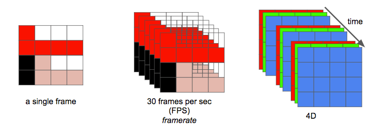
Otra propiedad de una images es la resolución, que es el número de píxeles en una dimensión. Frecuentemente es presentado como ancho × alto (width × height), por ejemplo, la siguiente imagen es 4×4.

Práctica: juguemos con una imagen y colores

Puedes jugar con una imagen y colores usando jupyter (python, numpy, matplotlib, etc).

También puedes aprender cómo funcionan los filtros de imágenes (edge detection, sharpen, blur...).

Trabajando con imágenes o vídeos, te encontrarás con otra propiedad llamada aspect ratio (relación de aspecto) que simplemente describe la relación proporcional que existe entre el ancho y alto de una imagen o píxel.

Cuando las personas dicen que una película o imagen es 16x9 usualmente se están refiriendo a la relación de aspecto de la pantalla (Display Aspect Ratio (DAR)), sin embargo podemos tener diferentes formas para cada píxel, a ello le llamamos relación de aspecto del píxel (Pixel Aspect Ratio (PAR)).

DVD es DAR 4:3

La resolución del formato de DVD es 704x480, igualmente mantiente una relación de aspecto (DAR) de 4:3 porque tiene PAR de 10:11 (704x10/480x11)

Finalmente, podemos definir a un vídeo como una sucesión de n cuadros en el tiempo, la cual la podemos definir como otra dimensión, n es el frame rate o cuadros por segundo (FPS, del inglés frames per second).

El número necesario de bits por segundo para mostrar un vídeo es llamado bit rate.

bit rate = ancho * alto * bit depth * FPS

Por ejemplo, un vídeo de 30 cuadros por segundo, 24 bits por píxel, 480x240 de resolución necesitaría de 82,944,000 bits por segundo o 82.944 Mbps (30x480x240x24) si no queremos aplicar ningún tipo de compresión.

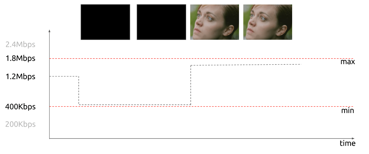
Cuando el bit rate es casi constante es llamado bit rate constante (CBR, del inglés constant bit rate), pero también puede ser variable por lo que lo llamaremos bit rate variable (VBR, del inglés variable bit rate).

La siguiente gráfica muestra como utilizando VBR no se necesita gastar demasiados bits para un cuadro es negro.

En otros tiempos, unos ingenieros idearon una técnica para duplicar la canidad de cuadros por segundo percividos en una pantalla sin consumir ancho de banda adicional. Esta técnica es conocida como vídeo entrelazado (interlaced video); básicamente envía la mitad de la pantalla en un "cuadro" y la otra mitad en el siguiente "cuadro".

Hoy en día, las pantallas representan imágenes principalmente utilizando la técnica de escaneo progresivo (progressive vídeo). El vídeo progresivo es una forma de mostrar, almacenar o transmitir imágenes en movimiento en la que todas las líneas de cada cuadro se dibujan en secuencia.

Ahora ya tenemos una idea acerca de cómo una imagen es representada digitalmente, cómo sus colores son codificados, cuántos bits por segundo necesitamos para mostrar un vídeo, si es constante (CBR) o variable (VBR), con una resolución dada a determinado frame rate y otros términos como entrelazado, PAR, etc.

Práctica: Verifiquemos las propiedades del vídeo

Puedes verificar la mayoría de las propiedades mencionadas con ffmpeg o mediainfo.

Eliminación de Redundancias

Aprendimos que no es factible utilizar vídeo sin ninguna compresión; un solo vídeo de una hora a una resolución de 720p y 30fps requeriría 278GB^*. Dado que utilizar únicamente algoritmos de compresión de datos sin pérdida como DEFLATE (utilizado en PKZIP, Gzip y PNG), no disminuiría suficientemente el ancho de banda necesario, debemos encontrar otras formas de comprimir el vídeo.

^* Encontramos este número multiplicando 1280 x 720 x 24 x 30 x 3600 (ancho, alto, bits por píxel, fps y tiempo en segundos).

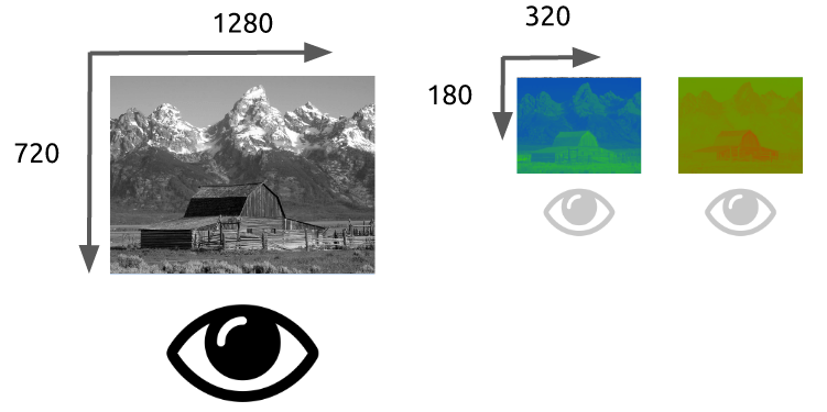
Para hacerlo, podemos aprovechar cómo funciona nuestra visión. Somos mejores para distinguir el brillo que los colores, las repeticiones en el tiempo, un vídeo contiene muchas imágenes con pocos cambios, y las repeticiones dentro de la imagen, cada cuadro también contiene muchas áreas que utilizan colores iguales o similares.

Colores, Luminancia y nuestros ojos

Nuestros ojos son más sensibles al brillo que a los colores, puedes comprobarlo por ti mismo, mira esta imagen.

Si no puedes ver que los colores de los cuadrados A y B son idénticos en el lado izquierdo, no te preocupes, es nuestro cerebro jugándonos una pasada para que prestemos más atención a la luz y la oscuridad que al color. Hay un conector, del mismo color, en el lado derecho para que nosotros (nuestro cerebro) podamos identificar fácilmente que, de hecho, son del mismo color.

Explicación simplista de cómo funcionan nuestros ojos El ojo es un órgano complejo, compuesto por muchas partes, pero principalmente nos interesan las células de conos y bastones. El ojo contiene alrededor de 120 millones de células de bastones y 6 millones de células de conos.

Para simplificar absurdamente, intentemos relacionar los colores y el brillo con las funciones de las partes del ojo. Los bastones son principalmente responsables del brillo, mientras que los conos son responsables del color. Hay tres tipos de conos, cada uno con un pigmento diferente, a saber: Tipo S (azul), Tipo M (verde) y Tipo L (rojos).

Dado que tenemos muchas más células de bastones (brillo) que células de conos (color), se puede inferir que somos más capaces de distinguir el contraste entre la luz y la oscuridad que los colores.

Funciones de sensibilidad al contraste

Los investigadores de psicología experimental y muchas otras disciplinas han desarrollado varias teorías sobre la visión humana. Una de ellas se llama funciones de sensibilidad al contraste. Están relacionadas con el espacio y el tiempo de la luz y su valor se presenta en una luz inicial dada, cuánto cambio se requiere antes de que un observador informe que ha habido un cambio. Observa el plural de la palabra "función", esto se debe a que podemos medir las funciones de sensibilidad al contraste no solo con blanco y negro, sino también con colores. El resultado de estos experimentos muestra que en la mayoría de los casos nuestros ojos son más sensibles al brillo que al color.

Una vez que sabemos que somos más sensibles a la luminancia (luma, el brillo en una imagen), podemos aprovecharlo.

Modelo de color

Primero aprendimos cómo funcionan las imágenes en color utilizando el modelo RGB, pero existen otros modelos también. De hecho, hay un modelo que separa la luminancia (brillo) de la crominancia (colores) y se conoce como YCbCr^*.

^* hay más modelos que hacen la misma separación.

Este modelo de color utiliza Y para representar el brillo y dos canales de color, Cb (croma azul) y Cr (croma rojo). El YCbCr se puede derivar a partir de RGB y también se puede convertir de nuevo a RGB. Utilizando este modelo, podemos crear imágenes a todo color, como podemos ver a continuación.

Conversiones entre YCbCr y RGB

Algunos pueden preguntarse, ¿cómo podemos producir todos los colores sin usar el verde?

Para responder a esta pregunta, vamos a realizar una conversión de RGB a YCbCr. Utilizaremos los coeficientes del estándar BT.601 que fue recomendado por el grupo ITU-R^*. El primer paso es calcular la luminancia, utilizaremos las constantes sugeridas por la ITU y sustituiremos los valores RGB.

Y = 0.299R + 0.587G + 0.114B

Una vez obtenida la luminancia, podemos separar los colores (croma azul y croma rojo):

Cb = 0.564(B - Y)
Cr = 0.713(R - Y)

Y también podemos covertirlo de vuelta e incluse obtener el verde utilizando YCbCr.

R = Y + 1.402Cr
B = Y + 1.772Cb
G = Y - 0.344Cb - 0.714Cr

^* Los grupos y estándares son comunes en el vídeo digital y suelen definir cuáles son los estándares, por ejemplo, ¿qué es 4K? ¿qué frecuencia de cuadro debemos usar? ¿resolución? ¿modelo de color?

Generalmente, las pantallas (monitores, televisores, etc.) utilizan solo el modelo RGB, organizado de diferentes maneras, como se muestra a continuación:

Chroma subsampling

With the image represented as luma and chroma components, we can take advantage of the human visual system's greater sensitivity for luma resolution rather than chroma to selectively remove information. Chroma subsampling is the technique of encoding images using less resolution for chroma than for luma.

How much should we reduce the chroma resolution?! It turns out that there are already some schemas that describe how to handle resolution and the merge (final color = Y + Cb + Cr).

These schemas are known as subsampling systems and are expressed as a 3 part ratio - a:x:y which defines the chroma resolution in relation to a a x 2 block of luma pixels.

a is the horizontal sampling reference (usually 4)
x is the number of chroma samples in the first row of a pixels (horizontal resolution in relation to a)
y is the number of changes of chroma samples between the first and seconds rows of a pixels.

An exception to this exists with 4:1:0, which provides a single chroma sample within each 4 x 4 block of luma resolution.

Common schemes used in modern codecs are: 4:4:4 (no subsampling), 4:2:2, 4:1:1, 4:2:0, 4:1:0 and 3:1:1.

You can follow some discussions to learn more about Chroma Subsampling.

YCbCr 4:2:0 merge

Here's a merged piece of an image using YCbCr 4:2:0, notice that we only spend 12 bits per pixel.

You can see the same image encoded by the main chroma subsampling types, images in the first row are the final YCbCr while the last row of images shows the chroma resolution. It's indeed a great win for such small loss.

Previously we had calculated that we needed 278GB of storage to keep a video file with one hour at 720p resolution and 30fps. If we use YCbCr 4:2:0 we can cut this size in half (139 GB)^* but it is still far from ideal.

^* we found this value by multiplying width, height, bits per pixel and fps. Previously we needed 24 bits, now we only need 12.

Hands-on: Check YCbCr histogram

You can check the YCbCr histogram with ffmpeg. This scene has a higher blue contribution, which is showed by the histogram.

Color, luma, luminance, gamma video review

Watch this incredible video explaining what is luma and learn about luminance, gamma, and color.

Hands-on: Check YCbCr intensity

You can visualize the Y intensity for a given line of a video using FFmpeg's oscilloscope filter.
ffplay -f lavfi -i 'testsrc2=size=1280x720:rate=30000/1001,format=yuv420p' -vf oscilloscope=x=0.5:y=200/720:s=1:c=1

Frame types

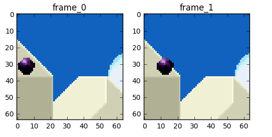
Now we can move on and try to eliminate the redundancy in time but before that let's establish some basic terminology. Suppose we have a movie with 30fps, here are its first 4 frames.

We can see lots of repetitions within frames like the blue background, it doesn't change from frame 0 to frame 3. To tackle this problem, we can abstractly categorize them as three types of frames.

I Frame (intra, keyframe)

An I-frame (reference, keyframe, intra) is a self-contained frame. It doesn't rely on anything to be rendered, an I-frame looks similar to a static photo. The first frame is usually an I-frame but we'll see I-frames inserted regularly among other types of frames.

P Frame (predicted)

A P-frame takes advantage of the fact that almost always the current picture can be rendered using the previous frame. For instance, in the second frame, the only change was the ball that moved forward. We can rebuild frame 1, only using the difference and referencing to the previous frame.

Hands-on: A video with a single I-frame

Since a P-frame uses less data why can't we encode an entire video with a single I-frame and all the rest being P-frames?

After you encoded this video, start to watch it and do a seek for an advanced part of the video, you'll notice it takes some time to really move to that part. That's because a P-frame needs a reference frame (I-frame for instance) to be rendered.

Another quick test you can do is to encode a video using a single I-Frame and then encode it inserting an I-frame each 2s and check the size of each rendition.

B Frame (bi-predictive)

What about referencing the past and future frames to provide even a better compression?! That's basically what a B-frame is.

<- ->

Hands-on: Compare videos with B-frame

You can generate two renditions, first with B-frames and other with no B-frames at all and check the size of the file as well as the quality.

Summary

These frames types are used to provide better compression. We'll look how this happens in the next section, but for now we can think of I-frame as expensive while P-frame is cheaper but the cheapest is the B-frame.

Temporal redundancy (inter prediction)

Let's explore the options we have to reduce the repetitions in time, this type of redundancy can be solved with techniques of inter prediction.

We will try to spend fewer bits to encode the sequence of frames 0 and 1.

One thing we can do it's a subtraction, we simply subtract frame 1 from frame 0 and we get just what we need to encode the residual.

But what if I tell you that there is a better method which uses even fewer bits?! First, let's treat the frame 0 as a collection of well-defined partitions and then we'll try to match the blocks from frame 0 on frame 1. We can think of it as motion estimation.

Wikipedia - block motion compensation

"Block motion compensation divides up the current frame into non-overlapping blocks, and the motion compensation vector tells where those blocks come from (a common misconception is that the previous frame is divided up into non-overlapping blocks, and the motion compensation vectors tell where those blocks move to). The source blocks typically overlap in the source frame. Some video compression algorithms assemble the current frame out of pieces of several different previously-transmitted frames."

We could estimate that the ball moved from x=0, y=25 to x=6, y=26, the x and y values are the motion vectors. One further step we can do to save bits is to encode only the motion vector difference between the last block position and the predicted, so the final motion vector would be x=6 (6-0), y=1 (26-25)

In a real-world situation, this ball would be sliced into n partitions but the process is the same.

The objects on the frame move in a 3D way, the ball can become smaller when it moves to the background. It's normal that we won't find the perfect match to the block we tried to find a match. Here's a superposed view of our estimation vs the real picture.

But we can see that when we apply motion estimation the data to encode is smaller than using simply delta frame techniques.

How real motion compensation would look

This technique is applied to all blocks, very often a ball would be partitioned in more than one block. Source: https://web.stanford.edu/class/ee398a/handouts/lectures/EE398a_MotionEstimation_2012.pdf

You can play around with these concepts using jupyter.

Hands-on: See the motion vectors

We can generate a video with the inter prediction (motion vectors) with ffmpeg.

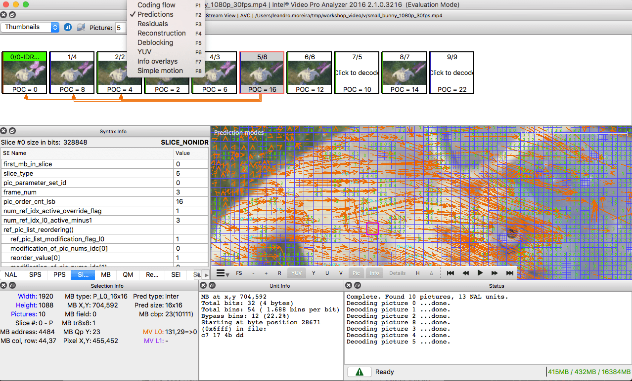
Or we can use the Intel Video Pro Analyzer (which is paid but there is a free trial version which limits you to only work with the first 10 frames).

Spatial redundancy (intra prediction)

If we analyze each frame in a video we'll see that there are also many areas that are correlated.

Let's walk through an example. This scene is mostly composed of blue and white colors.

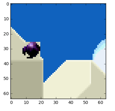
This is an I-frame and we can't use previous frames to predict from but we still can compress it. We will encode the red block selection. If we look at its neighbors, we can estimate that there is a trend of colors around it.

We will predict that the frame will continue to spread the colors vertically, it means that the colors of the unknown pixels will hold the values of its neighbors.

Our prediction can be wrong, for that reason we need to apply this technique (intra prediction) and then subtract the real values which gives us the residual block, resulting in a much more compressible matrix compared to the original.

There are many different types of this sort of prediction. The one you see pictured here is a form of straight planar prediction, where the pixels from the row above the block are copied row to row within the block. Planar prediction also can involve an angular component, where pixels from both the left and the top are used to help predict the current block. And there is also DC prediction, which involves taking the average of the samples right above and to the left of the block.

Hands-on: Check intra predictions

You can generate a video with macro blocks and their predictions with ffmpeg. Please check the ffmpeg documentation to understand the meaning of each block color.

Or we can use the Intel Video Pro Analyzer (which is paid but there is a free trial version which limits you to only work with the first 10 frames).

How does a video codec work?

What? Why? How?

What? It's a piece of software / hardware that compresses or decompresses digital video. Why? Market and society demands higher quality videos with limited bandwidth or storage. Remember when we calculated the needed bandwidth for 30 frames per second, 24 bits per pixel, resolution of a 480x240 video? It was 82.944 Mbps with no compression applied. It's the only way to deliver HD/FullHD/4K in TVs and the Internet. How? We'll take a brief look at the major techniques here.

CODEC vs Container

One common mistake that beginners often do is to confuse digital video CODEC and digital video container. We can think of containers as a wrapper format which contains metadata of the video (and possible audio too), and the compressed video can be seen as its payload.

Usually, the extension of a video file defines its video container. For instance, the file video.mp4 is probably a MPEG-4 Part 14 container and a file named video.mkv it's probably a matroska. To be completely sure about the codec and container format we can use ffmpeg or mediainfo.

History

Before we jump into the inner workings of a generic codec, let's look back to understand a little better about some old video codecs.

The video codec H.261 was born in 1990 (technically 1988), and it was designed to work with data rates of 64 kbit/s. It already uses ideas such as chroma subsampling, macro block, etc. In the year of 1995, the H.263 video codec standard was published and continued to be extended until 2001.

In 2003 the first version of H.264/AVC was completed. In the same year, On2 Technologies (formerly known as the Duck Corporation) released their video codec as a royalty-free lossy video compression called VP3. In 2008, Google bought this company, releasing VP8 in the same year. In December of 2012, Google released the VP9 and it's supported by roughly ¾ of the browser market (mobile included).

AV1 is a new royalty-free and open source video codec that's being designed by the Alliance for Open Media (AOMedia), which is composed of the companies: Google, Mozilla, Microsoft, Amazon, Netflix, AMD, ARM, NVidia, Intel and Cisco among others. The first version 0.1.0 of the reference codec was published on April 7, 2016.

The birth of AV1

Early 2015, Google was working on VP10, Xiph (Mozilla) was working on Daala and Cisco open-sourced its royalty-free video codec called Thor.

Then MPEG LA first announced annual caps for HEVC (H.265) and fees 8 times higher than H.264 but soon they changed the rules again:

no annual cap,

content fee (0.5% of revenue) and

per-unit fees about 10 times higher than h264.

The alliance for open media was created by companies from hardware manufacturer (Intel, AMD, ARM , Nvidia, Cisco), content delivery (Google, Netflix, Amazon), browser maintainers (Google, Mozilla), and others.

The companies had a common goal, a royalty-free video codec and then AV1 was born with a much simpler patent license. Timothy B. Terriberry did an awesome presentation, which is the source of this section, about the AV1 conception, license model and its current state.

You'll be surprised to know that you can analyze the AV1 codec through your browser, go to https://arewecompressedyet.com/analyzer/

PS: If you want to learn more about the history of the codecs you must learn the basics behind video compression patents.

A generic codec

We're going to introduce the main mechanics behind a generic video codec but most of these concepts are useful and used in modern codecs such as VP9, AV1 and HEVC. Be sure to understand that we're going to simplify things a LOT. Sometimes we'll use a real example (mostly H.264) to demonstrate a technique.

1st step - picture partitioning

The first step is to divide the frame into several partitions, sub-partitions and beyond.

But why? There are many reasons, for instance, when we split the picture we can work the predictions more precisely, using small partitions for the small moving parts while using bigger partitions to a static background.

Usually, the CODECs organize these partitions into slices (or tiles), macro (or coding tree units) and many sub-partitions. The max size of these partitions varies, HEVC sets 64x64 while AVC uses 16x16 but the sub-partitions can reach sizes of 4x4.

Remember that we learned how frames are typed?! Well, you can apply those ideas to blocks too, therefore we can have I-Slice, B-Slice, I-Macroblock and etc.

Hands-on: Check partitions

We can also use the Intel Video Pro Analyzer (which is paid but there is a free trial version which limits you to only work with the first 10 frames). Here are VP9 partitions analyzed.

2nd step - predictions

Once we have the partitions, we can make predictions over them. For the inter prediction we need to send the motion vectors and the residual and the intra prediction we'll send the prediction direction and the residual as well.

3rd step - transform

After we get the residual block (predicted partition - real partition), we can transform it in a way that lets us know which pixels we can discard while keeping the overall quality. There are some transformations for this exact behavior.

Although there are other transformations, we'll look more closely at the discrete cosine transform (DCT). The DCT main features are:

converts blocks of pixels into same-sized blocks of frequency coefficients.
compacts energy, making it easy to eliminate spatial redundancy.
is reversible, a.k.a. you can reverse to pixels.

On 2 Feb 2017, Cintra, R. J. and Bayer, F. M have published their paper DCT-like Transform for Image Compression Requires 14 Additions Only.

Don't worry if you didn't understand the benefits from every bullet point, we'll try to make some experiments in order to see the real value from it.

Let's take the following block of pixels (8x8):

Which renders to the following block image (8x8):

When we apply the DCT over this block of pixels and we get the block of coefficients (8x8):

And if we render this block of coefficients, we'll get this image:

As you can see it looks nothing like the original image, we might notice that the first coefficient is very different from all the others. This first coefficient is known as the DC coefficient which represents all the samples in the input array, something similar to an average.

This block of coefficients has an interesting property which is that it separates the high-frequency components from the low frequency.

In an image, most of the energy will be concentrated in the lower frequencies, so if we transform an image into its frequency components and throw away the higher frequency coefficients, we can reduce the amount of data needed to describe the image without sacrificing too much image quality.

frequency means how fast a signal is changing

Let's try to apply the knowledge we acquired in the test by converting the original image to its frequency (block of coefficients) using DCT and then throwing away part of the least important coefficients.

First, we convert it to its frequency domain.

Next, we discard part (67%) of the coefficients, mostly the bottom right part of it.

Finally, we reconstruct the image from this discarded block of coefficients (remember, it needs to be reversible) and compare it to the original.

As we can see it resembles the original image but it introduced lots of differences from the original, we throw away 67.1875% and we still were able to get at least something similar to the original. We could more intelligently discard the coefficients to have a better image quality but that's the next topic.

Each coefficient is formed using all the pixels

It's important to note that each coefficient doesn't directly map to a single pixel but it's a weighted sum of all pixels. This amazing graph shows how the first and second coefficient is calculated, using weights which are unique for each index.

Source: https://web.archive.org/web/20150129171151/https://www.iem.thm.de/telekom-labor/zinke/mk/mpeg2beg/whatisit.htm

You can also try to visualize the DCT by looking at a simple image formation over the DCT basis. For instance, here's the A character being formed using each coefficient weight.

Hands-on: throwing away different coefficients

You can play around with the DCT transform.

4th step - quantization

When we throw away some of the coefficients, in the last step (transform), we kinda did some form of quantization. This step is where we chose to lose information (the lossy part) or in simple terms, we'll quantize coefficients to achieve compression.

How can we quantize a block of coefficients? One simple method would be a uniform quantization, where we take a block, divide it by a single value (10) and round this value.

How can we reverse (re-quantize) this block of coefficients? We can do that by multiplying the same value (10) we divide it first.

This approach isn't the best because it doesn't take into account the importance of each coefficient, we could use a matrix of quantizers instead of a single value, this matrix can exploit the property of the DCT, quantizing most the bottom right and less the upper left, the JPEG uses a similar approach, you can check source code to see this matrix.

Hands-on: quantization

You can play around with the quantization.

5th step - entropy coding

After we quantized the data (image blocks/slices/frames) we still can compress it in a lossless way. There are many ways (algorithms) to compress data. We're going to briefly experience some of them, for a deeper understanding you can read the amazing book Understanding Compression: Data Compression for Modern Developers.

VLC coding:

Let's suppose we have a stream of the symbols: a, e, r and t and their probability (from 0 to 1) is represented by this table.

	a	e	r	t
probability	0.3	0.3	0.2	0.2

We can assign unique binary codes (preferable small) to the most probable and bigger codes to the least probable ones.

	a	e	r	t
probability	0.3	0.3	0.2	0.2
binary code	0	10	110	1110

Let's compress the stream eat, assuming we would spend 8 bits for each symbol, we would spend 24 bits without any compression. But in case we replace each symbol for its code we can save space.

The first step is to encode the symbol e which is 10 and the second symbol is a which is added (not in a mathematical way) [10][0] and finally the third symbol t which makes our final compressed bitstream to be [10][0][1110] or 1001110 which only requires 7 bits (3.4 times less space than the original).

Notice that each code must be a unique prefixed code Huffman can help you to find these numbers. Though it has some issues there are video codecs that still offers this method and it's the algorithm for many applications which requires compression.

Both encoder and decoder must know the symbol table with its code, therefore, you need to send the table too.

Arithmetic coding:

Let's suppose we have a stream of the symbols: a, e, r, s and t and their probability is represented by this table.

	a	e	r	s	t
probability	0.3	0.3	0.15	0.05	0.2

With this table in mind, we can build ranges containing all the possible symbols sorted by the most frequents.

Now let's encode the stream eat, we pick the first symbol e which is located within the subrange 0.3 to 0.6 (but not included) and we take this subrange and split it again using the same proportions used before but within this new range.

Let's continue to encode our stream eat, now we take the second symbol a which is within the new subrange 0.3 to 0.39 and then we take our last symbol t and we do the same process again and we get the last subrange 0.354 to 0.372.

We just need to pick a number within the last subrange 0.354 to 0.372, let's choose 0.36 but we could choose any number within this subrange. With only this number we'll be able to recover our original stream eat. If you think about it, it's like if we were drawing a line within ranges of ranges to encode our stream.

The reverse process (A.K.A. decoding) is equally easy, with our number 0.36 and our original range we can run the same process but now using this number to reveal the stream encoded behind this number.

With the first range, we notice that our number fits at the slice, therefore, it's our first symbol, now we split this subrange again, doing the same process as before, and we'll notice that 0.36 fits the symbol a and after we repeat the process we came to the last symbol t (forming our original encoded stream eat).

Both encoder and decoder must know the symbol probability table, therefore you need to send the table.

Pretty neat, isn't it? People are damn smart to come up with a such solution, some video codecs use this technique (or at least offer it as an option).

The idea is to lossless compress the quantized bitstream, for sure this article is missing tons of details, reasons, trade-offs and etc. But you should learn more as a developer. Newer codecs are trying to use different entropy coding algorithms like ANS.

Hands-on: CABAC vs CAVLC

You can generate two streams, one with CABAC and other with CAVLC and compare the time it took to generate each of them as well as the final size.

6th step - bitstream format

After we did all these steps we need to pack the compressed frames and context to these steps. We need to explicitly inform to the decoder about the decisions taken by the encoder, such as bit depth, color space, resolution, predictions info (motion vectors, intra prediction direction), profile, level, frame rate, frame type, frame number and much more.

We're going to study, superficially, the H.264 bitstream. Our first step is to generate a minimal H.264 ^* bitstream, we can do that using our own repository and ffmpeg.

./s/ffmpeg -i /files/i/minimal.png -pix_fmt yuv420p /files/v/minimal_yuv420.h264

^* ffmpeg adds, by default, all the encoding parameter as a SEI NAL, soon we'll define what is a NAL.

This command will generate a raw h264 bitstream with a single frame, 64x64, with color space yuv420 and using the following image as the frame.

H.264 bitstream

The AVC (H.264) standard defines that the information will be sent in macro frames (in the network sense), called NAL (Network Abstraction Layer). The main goal of the NAL is the provision of a "network-friendly" video representation, this standard must work on TVs (stream based), the Internet (packet based) among others.

There is a synchronization marker to define the boundaries of the NAL's units. Each synchronization marker holds a value of 0x00 0x00 0x01 except to the very first one which is 0x00 0x00 0x00 0x01. If we run the hexdump on the generated h264 bitstream, we can identify at least three NALs in the beginning of the file.

As we said before, the decoder needs to know not only the picture data but also the details of the video, frame, colors, used parameters, and others. The first byte of each NAL defines its category and type.

NAL type id	Description
0	Undefined
1	Coded slice of a non-IDR picture
2	Coded slice data partition A
3	Coded slice data partition B
4	Coded slice data partition C
5	IDR Coded slice of an IDR picture
6	SEI Supplemental enhancement information
7	SPS Sequence parameter set
8	PPS Picture parameter set
9	Access unit delimiter
10	End of sequence
11	End of stream
...	...

Usually, the first NAL of a bitstream is a SPS, this type of NAL is responsible for informing the general encoding variables like profile, level, resolution and others.

If we skip the first synchronization marker we can decode the first byte to know what type of NAL is the first one.

For instance the first byte after the synchronization marker is 01100111, where the first bit (0) is to the field forbidden_zero_bit, the next 2 bits (11) tell us the field nal_ref_idc which indicates whether this NAL is a reference field or not and the rest 5 bits (00111) inform us the field nal_unit_type, in this case, it's a SPS (7) NAL unit.

The second byte (binary=01100100, hex=0x64, dec=100) of an SPS NAL is the field profile_idc which shows the profile that the encoder has used, in this case, we used the high profile. Also the third byte contains several flags which determine the exact profile (like constrained or progressive). But in our case the third byte is 0x00 and therefore the encoder has used just high profile.

When we read the H.264 bitstream spec for an SPS NAL we'll find many values for the parameter name, category and a description, for instance, let's look at pic_width_in_mbs_minus_1 and pic_height_in_map_units_minus_1 fields.

Parameter name	Category	Description
pic_width_in_mbs_minus_1	0	ue(v)
pic_height_in_map_units_minus_1	0	ue(v)

ue(v): unsigned integer Exp-Golomb-coded

If we do some math with the value of these fields we will end up with the resolution. We can represent a 1920 x 1080 using a pic_width_in_mbs_minus_1 with the value of 119 ( (119 + 1) * macroblock_size = 120 * 16 = 1920) , again saving space, instead of encode 1920 we did it with 119.

If we continue to examine our created video with a binary view (ex: xxd -b -c 11 v/minimal_yuv420.h264), we can skip to the last NAL which is the frame itself.

We can see its first 6 bytes values: 01100101 10001000 10000100 00000000 00100001 11111111. As we already know the first byte tell us about what type of NAL it is, in this case, (00101) it's an IDR Slice (5) and we can further inspect it:

Using the spec info we can decode what type of slice (slice_type), the frame number (frame_num) among others important fields.

In order to get the values of some fields (ue(v), me(v), se(v) or te(v)) we need to decode it using a special decoder called Exponential-Golomb, this method is very efficient to encode variable values, mostly when there are many default values.

The values of slice_type and frame_num of this video are 7 (I slice) and 0 (the first frame).

We can see the bitstream as a protocol and if you want or need to learn more about this bitstream please refer to the ITU H.264 spec. Here's a macro diagram which shows where the picture data (compressed YUV) resides.

We can explore others bitstreams like the VP9 bitstream, H.265 (HEVC) or even our new best friend AV1 bitstream, do they all look similar? No, but once you learned one you can easily get the others.

Hands-on: Inspect the H.264 bitstream

We can generate a single frame video and use mediainfo to inspect its H.264 bitstream. In fact, you can even see the source code that parses h264 (AVC) bitstream.

We can also use the Intel Video Pro Analyzer which is paid but there is a free trial version which limits you to only work with the first 10 frames but that's okay for learning purposes.

Review

We'll notice that many of the modern codecs uses this same model we learned. In fact, let's look at the Thor video codec block diagram, it contains all the steps we studied. The idea is that you now should be able to at least understand better the innovations and papers for the area.

Previously we had calculated that we needed 139GB of storage to keep a video file with one hour at 720p resolution and 30fps if we use the techniques we learned here, like inter and intra prediction, transform, quantization, entropy coding and other we can achieve, assuming we are spending 0.031 bit per pixel, the same perceivable quality video requiring only 367.82MB vs 139GB of store.

We choose to use 0.031 bit per pixel based on the example video provided here.

How does H.265 achieve a better compression ratio than H.264?

Now that we know more about how codecs work, then it is easy to understand how new codecs are able to deliver higher resolutions with fewer bits.

We will compare AVC and HEVC, let's keep in mind that it is almost always a trade-off between more CPU cycles (complexity) and compression rate.

HEVC has bigger and more partitions (and sub-partitions) options than AVC, more intra predictions directions/angles, improved entropy coding and more, all these improvements made H.265 capable to compress 50% more than H.264.

Online streaming

General architecture

[TODO]

Progressive download and adaptive streaming

[TODO]

Content protection

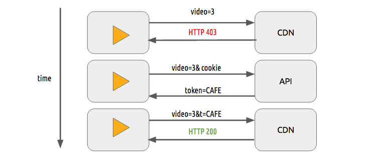
We can use a simple token system to protect the content. The user without a token tries to request a video and the CDN forbids her or him while a user with a valid token can play the content, it works pretty similarly to most of the web authentication systems.

The sole use of this token system still allows a user to download a video and distribute it. Then the DRM (digital rights management) systems can be used to try to avoid this.

In real life production systems, people often use both techniques to provide authorization and authentication.

DRM

Main systems

What?

DRM means Digital rights management, it's a way to provide copyright protection for digital media, for instance, digital video and audio. Although it's used in many places it's not universally accepted.

Why?

Content creator (mostly studios) want to protect its intelectual property against copy to prevent unauthorized redistribution of digital media.

How?

We're going to describe an abstract and generic form of DRM in a very simplified way.

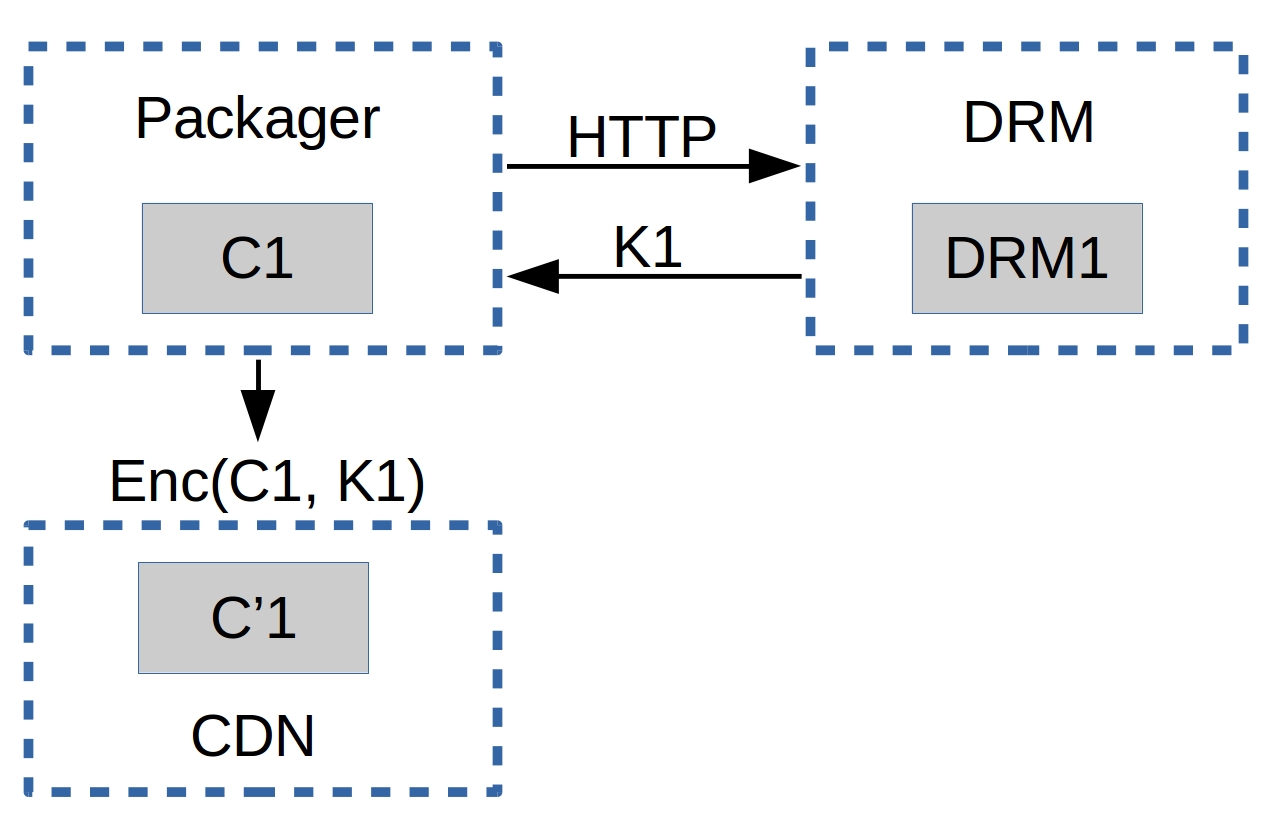
Given a content C1 (i.e. an hls or dash video streaming), with a player P1 (i.e. shaka-clappr, exo-player or ios) in a device D1 (i.e. a smartphone, TV, tablet or desktop/notebook) using a DRM system DRM1 (widevine, playready or FairPlay).

The content C1 is encrypted with a symmetric-key K1 from the system DRM1, generating the encrypted content C'1.

The player P1, of a device D1, has two keys (asymmetric), a private key PRK1 (this key is protected¹ and only known by D1) and a public key PUK1.

¹protected: this protection can be via hardware, for instance, this key can be stored inside a special (read-only) chip that works like a black-box to provide decryption, or by software (less safe), the DRM system provides means to know which type of protection a given device has.

When the player P1 wants to play the content C'1, it needs to deal with the DRM system DRM1, giving its public key PUK1. The DRM system DRM1 returns the key K1 encrypted with the client''s public key PUK1. In theory, this response is something that only D1 is capable of decrypting.

K1P1D1 = enc(K1, PUK1)

P1 uses its DRM local system (it could be a SOC, a specialized hardware or software), this system is able to decrypt the content using its private key PRK1, it can decrypt the symmetric-key K1 from the K1P1D1 and play C'1. At best case, the keys are not exposed through RAM.

K1 = dec(K1P1D1, PRK1)

P1.play(dec(C'1, K1))

How to use jupyter

Make sure you have docker installed and just run ./s/start_jupyter.sh and follow the instructions on the terminal.

Conferences

DEMUXED - you can check the last 2 events presentations..

References

The richest content is here, it's where all the info we saw in this text was extracted, based or inspired by. You can deepen your knowledge with these amazing links, books, videos and etc.

Online Courses and Tutorials:

Books:

Onboarding material:

Bitstream Specifications:

Software:

Non-ITU Codecs:

Encoding Concepts:

Video Sequences for Testing:

Miscellaneous:

67 KiB Raw Blame History Unescape Escape